Introduction
As you walk into a library you're greeted with a new arrivals section. You take an initial look around you see a children's section, DVDs, fiction, magazines, and much more. You came to the library with two goals.
The first is to find A Brief History of Time by Stephen Hawking. You don't come to the library very often so you're not really sure where it might be. So what do you do? You go to the computer, type in the book title, and it gives you back the Dewey Decimal. You use it to pinpoint exactly where the book is located.
Your second goal is to find general information on the state of computer hardware in 2002 for some research you're doing on the effects of the Dot-com bubble. You remember that as you walked in you saw a magazines section which makes you wonder if they might have PC Magazine from that time. You walk over and there are tons of bins of magazines, but an image of a computer catches your eye on one of the magazines! Success, you found the PC Magazine bin. They are ordered chronologically by month so you quickly pull out some issues from 2002.
Imagine if the media in the library was concentrated in one massive pile; it would be nearly impossible to find what you're looking for in a reasonable amount of time. What have your librarians done to enable you to quickly find what you're looking for? The answer should be obvious: they've organized everything such that your intuition guides you straight to your answer. In the first case you knew exactly what you were looking for, so the library's system let you pinpoint the exact book immediately. In the second case you weren't as specific, but the library's organization still let you find what you were looking for quickly.
Now imagine you're Google who knows of and has data on 36 trillion web pages. Your goal is to facilitate a user
finding a some webpage that they have in mind. How do you go from someone typing in a search query in
the Google box to getting results relevant to what they had in mind when they made that query and do so
quickly?
We'll explore answering this question by applying the concepts of Information Retrieval
Salton, G. (1968). Automatic information organization and retrieval. New York: McGraw-Hill.
High-Level Architecture of a Search Engine
Given our collection of data and an arbitrary inquiry, our goal is to enable efficient retrieval of the most relevant documents to that inquiry. In order to describe each component that goes into achieving this goal, we must note that each is strongly impacted by all the others. Decisions made in one component, directly affect decisions made downstream. With this in mind, we start with the two key components of a search engine: indexing and query processing. Indexing can be further broken down into processing data and the creation of an index, the core data structure of a search engine. Query processing can be broken down into processing user queries, ranking documents, and evaluation.
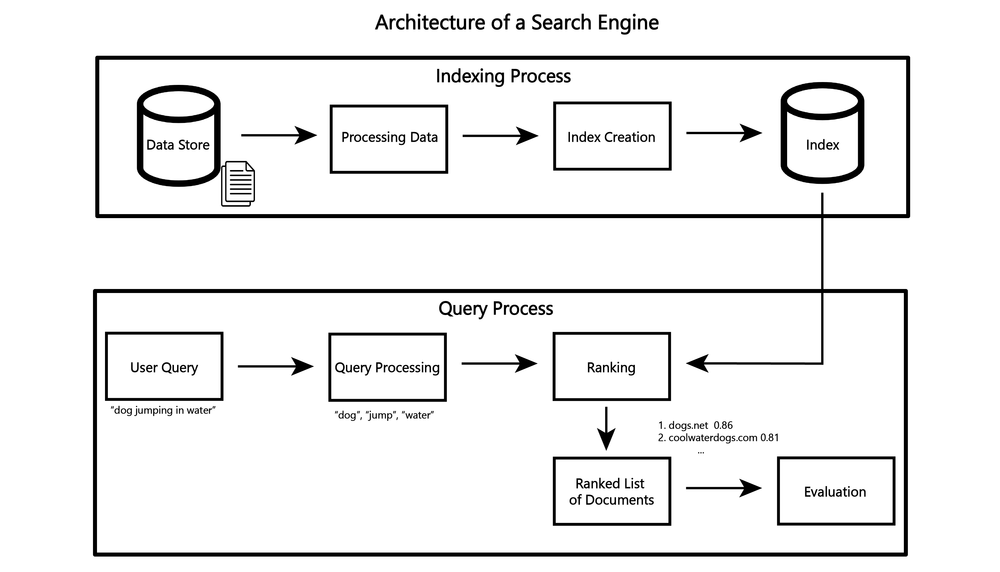
Before we can ask a user for a query and give them results, we must have data alongside a means of efficiently searching through it. The goal of the indexing process is to create a data structure that enables fast lookup of each document's features. The processing data component will take our raw documents and transform them into features that will represent its contents. The index creation component will then take the features and create the index data structure. More details will come later, but it is important to remember now that the index can consist of many different data structures and it must be able to be updated efficiently.
The query process takes a user's input and returns a list of documents either for the user's use or further evaluation (as in evaluating the effectiveness of our search engine). After taking in the user query, the search engine processes and enhances it in ways to enable better ranking of documents that might be relevant to that query. The ranking component will then take the processed query alongside the index and produce a ranked list of documents that it deems most relevant to the user's query. Finally, the evaluation component is something that is not seen by the user, but allows the creators of the search engine to be able to access its effectiveness.
Creating Our Own Search Engine
An Application for Twitter
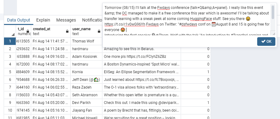
The search problem we explore in this article is searching over a collection of machine learning related tweets. We have a collection of tweets accumulated since May 2019 from the home timeline of the following Twitter account. We will refer to each "tweet" as a document, and each document consists of the following contents:
- Raw text of the tweet
- Note that if a tweet originally had a URL, we attempt to transform that URL into that URL's title and description HTML tags.
- Display name of the tweet's author
- Creation time of the tweet
- An indicator if the tweet is relevant or not to the topics machine learning and data science
The goals one might have when searching this collection are broad, some specific use cases we consider are finding:
- News, information, or research on a particular topic in ML
- Tutorials, talks, articles on a particular topic, potentially from a particular user
- A specific tweet you saw
- Any of the above tailored to a specific time frame (i.e. from October 2019)
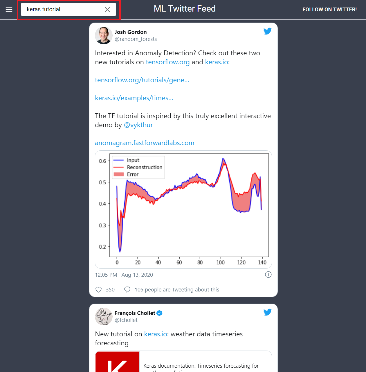
The interface for the user to let us know of what they want to find, is exactly what one would expect. It is a simple search box where a user can type arbitrary natural language.
Processing Data Indexing Ranking
We mentioned previously that each component is strongly impacted by all the others. The first step in our architecture is to process our raw documents. But before we process data, we have to know how that processed data will end up as features in our index, or else how do we know what to do with it?
But before we create an index, we need to know how we are going to use the features that we have for each document. We know they should be used to score and rank the documents represented in it. Therefore we first describe the methods for scoring our documents.
The main piece of our raw data that will enable us to find what we're looking for is the raw text of the tweet. Every other feature can be thought of as enhancing the quality of our ranking, rather than discovery of what documents might actually be relevant. Retrieval models usually focus on text, since it is what is common among a wide variety of retrieval tasks. Figuring out how to incorporate other domain-specific features is harder to generalize, as one might expect.
Retrieval Models - BM25
Determining how best to go from what information a person wants to retrieve, to some formally computable model
has been an area of research for decades, since the late 1950s
DOI:http://dx.doi.org/10.1016/j.ipm.2007.02.012
DOI:http://dx.doi.org/10.1561/1500000019
https://wikimedia-research.github.io/Discovery-Search-Test-BM25/
The most important aspect of understanding BM25 is that it is a "bag of words" model. This means it will calculate a score based on individual tokens within the document and considers them independently. The user query is what drives BM25, which needs to be tokenized into individual words. We will go into more detail on how this is done towards the end of the article. For now, it suffices to know that BM25 will consider each token in the query one at a time.
Given various statistics about individual terms across your collection of documents and your tokenized query, the BM25 scoring function will create a score for one document at a time and is defined as follows:
-
i := i^{th} \: term \: in \: tokenized \: query \: Q -
N := number \: of \: docs \: in \: the \: collection -
n_i := number \: of \: docs \: containing \: term \: i -
K := k_i((1-b)+b(\frac{dl}{avgdl})) -
k_1 := constant, \: hyperparameter -
b := constant, \: hyperparameter -
dl := length \: of \: the \: document -
avgdl := average \: length \: of \: a \: document \: in \: the \: collection -
f_i := frequency \: of \: term \: i \: in \: the \: document -
qf_i := frequency \: of \: term \: i \: in \: the \: query
Note that BM25 values are unbounded and can be negative (due to the log).
For every term in the query, we will first calculate the inverse document frequency, or IDF, component. This
first
component of the summation is penalizing words in the query that occur in many documents. For example, if the
number of documents containing a term,
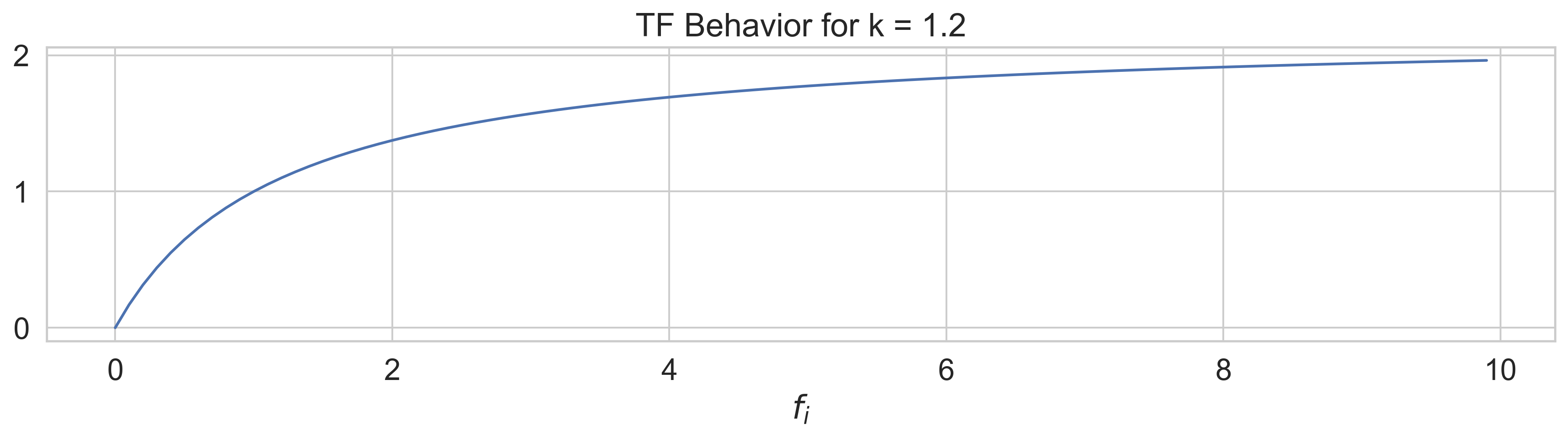
The second component of the summation is the term-frequency, TF. If we disregard the constants that are fixed for
every document, we are left with just
The third component serves to factor in the frequency of terms in the query. If
In literature the best default parameters are usually set to be
We set
In summary, what does BM25 get us? It provides us a way to take information about tokenized text in our documents and output a score. It uses information on how often terms occur in the entire collection, how often they occur in the current document, and how often words occur in our query. These three components combined give us a great measure of topical relevance, or relevance of documents based on the content in the query and document.
Other Features
As noted before, we have more data than only the raw text of tweets. We incorporate our domain specific features alongside BM25 to create a single model that will get us more relevant results than only using BM25 as our scoring function.
URLs: A feature we compute is the number of URLs that a tweet contains. Oftentimes when we search in this context, we want more information about a topic or a reference to a more detailed resource. Therefore, a tweet with a URL linking to another resource is likely to be more relevant than a tweet that is just simple text. Also of note is that most tweets will have between 0-3 URLs and having any above 2 does not contribute much further to the relevance.
Temporal: In most cases, given the choice between two similar resources on the same topic, we would want the more recent one. Therefore, we will give a small boost in ranking to tweets that were created more recently. We do this by assigning each tweet a value from 1 to the number of tweets in the collection, where the newest tweet has the highest value.
Relevance to Machine Learning: We use a binary value to indicate if the tweet is relevant or not to the topics of machine learning and data science. Another choice would have been to restrict completely any non-relevant tweets from showing in search results. However, this indicator feature is imperfect and is subjective so we opt to instead use this as a feature to push the non-relevant tweets down the ranking rather than completely eliminating them from search results.
Final Weighting
Given all these features and BM25 with each having different distributions and possible scales, we need a way to combine them into one score. Our goal will be to scale the final score so that it is between 0 and 1, and that the final score will be a linear combination of each feature, including BM25.
Sigmoid is a function that has the characteristic "S-curve", and the logistic function is a specific example that
maps arbitrary numbers to the range 0 to 1.
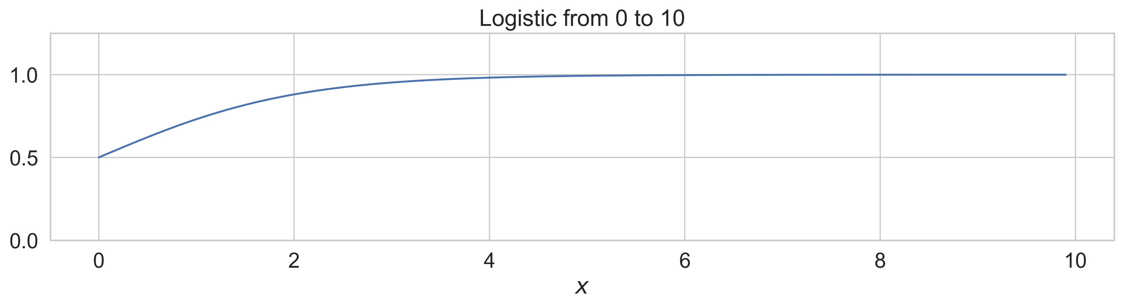
Once the values are higher than 5 or so, the difference between outputs of the function are minimal. This
property is desirable for URLs since they range mostly from 0 to 3, but for BM25 and temporal this poses an issue
since their values tend to range much higher. We still want to be able to discriminate between values in the upper
part of the range. So what we did to solve this is to scale the logistic function as follows:
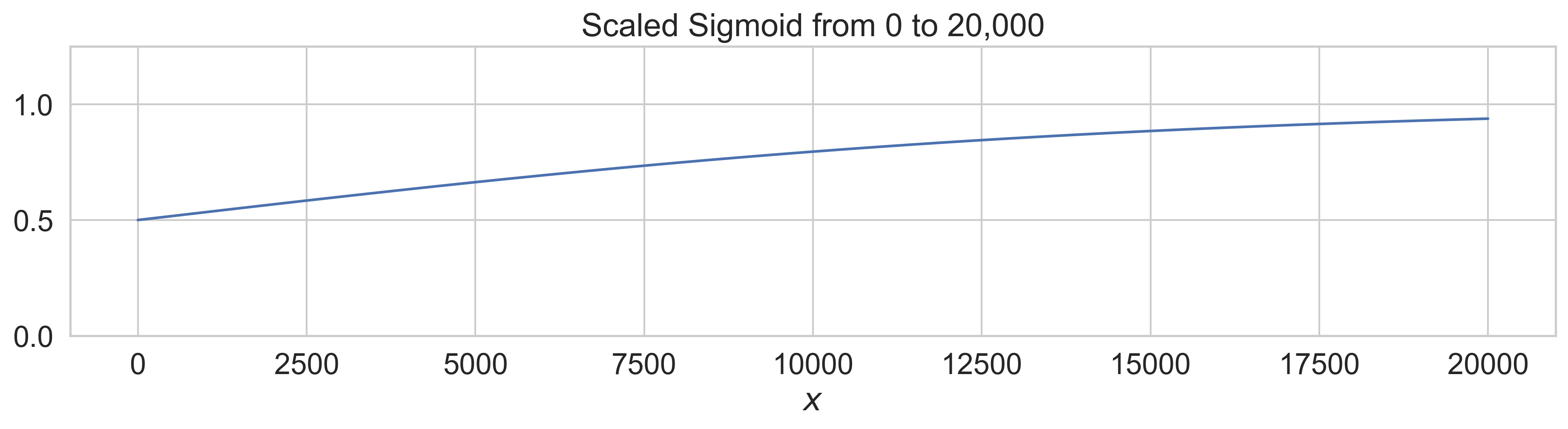
The behavior of this function is that for whatever value
Finally, we can create our linear combination of all the features to create a single score as follows:
The weights for each feature were set in such a way that reflects our intuition of their impact on document relevance. BM25 accounts for retrieving by the actual contents, so its weight is the majority. Predictions are also highly weighted because we want to focus on results that are relevant to machine learning. URLs are also fairly important to relevance so they have a weight of 15%. Lastly, we want recency to only nudge results in the ranking slightly, so we set that weight to 10%.
Processing Text
Now that we know our ranking function requires our documents to be tokenized and what affects the ranking, we turn to processing each document's raw text. The steps we take here are not entirely unique to search engines and could likely be applied to other problems in natural language processing using this dataset. Similarly, more sophisticated methods of processing text not mentioned here could also be applied to this problem.
Username: To allow search by the author of a tweet, we concatenate the username and tweet's text together.
Stop words: Stop words are words that get filtered out when processing text. Generally, they are common words that do not convey much meaning on their own. Since BM25 is a bag-of-words model, it makes sense to remove them from our text because we do not consider the associations between words. We used the stop word list from the NLP library spaCy. A full list of stop words it removes in English can be found on Github.
Punctuation and symbols: Similar to stop words, we remove any non-word symbols since they do not convey much meaning on their own. Removing extraneous tokens does not have a huge impact, but it does ensure our statistics like document length are more accurate and consistent.
Lemmatization: The lemma of a word is its base, or dictionary form. Lemmatization is the process of
algorithmically converting tokens to their lemmas based on part of speech and potentially the context of the word.
We used the spaCy Lemmatizer supports simple
part-of-speech-sensitive suffix rules and lookup tables.
For example if we provide it the string "search searching searches searched", it outputs the tokens
["search",
"searching", "search", "search"]. If we just provide it the string "searching" then it outputs ["search"] as the
tokens. In the first case "searching" interestingly stays the same. This occurs because in the first case spaCy
detected it to be a noun in that sentence, rather than as a verb.
Remove URLs: All URLs in tweets are always converted to be in Twitter's shortened format. This means that each URL is effectively unique, so it does not convey any meaning and thus it is removed. Note that we do count the number of occurrences of URLs and in most cases have appended onto the text the URL's resolved title and description.
@ mentions: When a tweet has an @ mention, it shows up in the raw text as the mentioned user's handle preceded by the '@' symbol. Someone using the search might want to find the tweets of particular users, but it is unlikely they would use the '@' symbol when doing so. As such, we remove the '@' character if it is the first character of any token.
Date of tweet: We often want to find information from a specific time frame, especially from a particular year, month, or even a specific day. To allow for search by temporal features, we tokenize the creation time of the tweet. The creation time of the tweet becomes three tokens, the full year, the full name of the month, and the day of the month.
Below we show an example of how an original tweet gets tokenized.

The tokens output by our text processing system is as follows: ['josh', 'gordon', 'check', 'new', 'amp', 'improve', 'load', 'image', 'tutorial', 'thank', 'amy', 'jang', 'show', 'way', 'load', 'dataset', 'keras.preprocesse', 'write', 'input', 'pipeline', 'scratch', 'w/', 'tensorflow', 'dataset', 'load', 'image', 'tensorflow', 'core', 'august', '16', '2020']
Note that the 'load', 'image', 'tensorflow', 'core' at the end of the list come from the title and description of the first URL in the tweet.
Index Creation
With our text processing pipeline and a definition of our ranking function, we now explain our index data structure. As a reminder to the reader, our ranking function requires us to have a lot of statistics about our documents available. As a review this info is summarized here:
- Total number of documents in the collection
- Average token count of documents in the collection
- For every document
- Number of URLs
- Relative time
- Frequency of terms in the documents
- Number of documents containing a particular term
Given that we need to respond to user's queries in real time, we need to look up this information in constant time. To store the frequency of terms in documents and the number of documents containing a particular term, we will use the data structure present in virtually every search engine, an inverted index. An inverted index is essentially a lookup table that maps terms to relevant data for that term. It is "inverted" because usually we would think of terms being a part of documents, so we would map documents to the terms it contains. However in this case, our terms are what we will use to lookup documents.All the other information we have does not depend on terms, so we can use a standard hashmap data structure to store it.
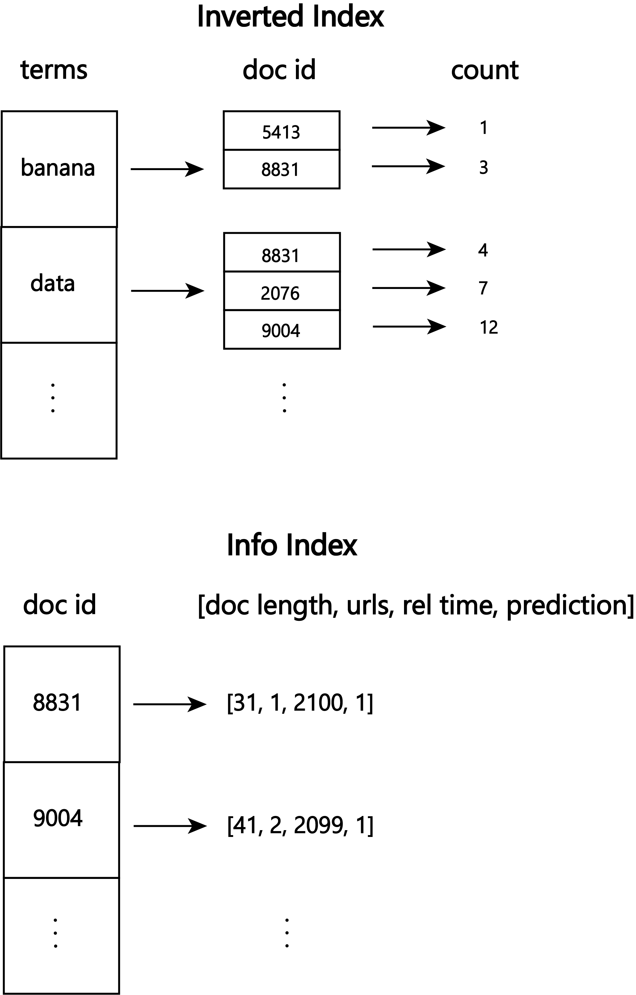
We map terms to a mapping of document id to the count of the term in that document. This allows us in constant time to get the number of documents containing that term (by looking at the number of doc id's for that term), and the count of that term in the document. As shown in the 'Info Index' figure, most of the other information we can store in a normal map of document id to the length of the document, how many urls it contains, its relative time to other tweets, and the indicator of relevancy.
Lastly, we keep track of the number of overall documents in the collection and the average of their lengths. The
average is updated using the following streaming average formula:
Query Processing
Using our index data structures, we can finally take a user query and generate a ranked list of results. We first must take the user's query and process it. This must be done in such a way that matches how we created our index to ensure we are looking up in our inverted index by the same tokens. Therefore, we take the same processing steps as we did during processing our text for indexing, like lemmatization and removing @ mentions.
Query Expansion: Query expansion is taking the original query, and manipulating or expanding it such that we get more relevant results to the user. One area query expansion can help with is misspellings. Another are words that are similar in meaning and are spelled similarly which occurs frequently in this domain. For example, the user may be interested in GANs, so they search "GAN". However, it turns out that oftentimes tweets instead contain the term "GANs" or are about the more specific "WGAN". To solve this, we find words in our index that are similar to a query token, and add those to our list of tokens we will use for ranking. The exact algorithm we use for finding words most similar to all of the other words in the index is Python's built in difflib library. The get_close_matches uses an algorithm that finds similar words by the notion of a "longest *contiguous* & junk-free matching subsequence". We chose to choose the three most similar words that are above the 0.8 score threshold. Currently in our system, if the query is "GAN" then our query will end up being tokenized into: ["gan", "wgan", "rgan"]. As the final step of the process, the query tokens are fed into the ranking function and we get our final ranked list!
Examples!
If you would like to see the results of this in practice for yourself and head over to https://mlfeed.tech. Type any query into the search box and enjoy!
Future Work
Improvements to search can be a lifetime of work and research in the field is ongoing, especially as it becomes more deeply integrated with natural language processing. Here we propose a few improvements that may improve our rankings.
Remove near duplicates: Users on Twitter tend to tweet about similar or identical things. We would want to remove any results from our ranking that are too similar to the ones higher in the ranking. One naive algorithm for this would be to vectorize each tweet, such as by using tf-idf. Then, we would go through the list of results, calculate the pairwise cosine similarity to every other tweet above in the ranking, and remove any result above a certain threshold. The downside of this is that it might be a fairly expensive operation to perform on demand.
Query expansion based on user data: A search engine like Google often determines query suggestions and expansion by using data about what other people have searched. For example, someone misspelled 'search' as 'saerch' in their first query, but then shortly after searches for 'search'. We can use that association to expand the query or even provide the user with spelling suggestions. Additionally, we could take advantage of popular queries. For every query we get, we might check our list of popular queries to see if there are any that are very similar in content to the new query we just got. If so, we could expand the new query by adding the popular one as well. For example, if many people search for "WGAN-GP", we might expand "WGAN" to also include "WGAN-GP" because the latter is popular and the text is very similar. Similarly, instead of being as intrusive, we could provide a "users also searched for" tip that lists all the queries that users also searched for that are close to the query the user searched for.
Concrete relevance data: We currently based many of our choices on strictly intuition, rather than formal metrics. Put another way, we did not optimize our choices based on any metric, but rather until the search results "looked good". With search engines being very subjective, this ends up being better than it sounds. However, it would be useful to formalize some query to document ranking mappings that we could calculate metrics like average precision or normalized DCG.
Conclusion
In this article we explored the fundamental principles of search engines to solve the problem of searching efficiently a collection of tweets. Each of these principles can be applied to a wide variety of other problems in information retrieval. While there will certainly be different choices made on a case by case, these same principles are what underpin every major application of retrieval from Google's web search to Windows desktop search to search on a social media platform like Facebook. The choices that can be made are limitless, so we focused on our particular problem of searching tweets in order to build the reader's intuition on how they can apply their domain knowledge to their own problem. The result is a foundation that can be used to build a search engine for any task.
If you enjoyed this article, consider reading my articles on Ensembling Forecasts AdaBoost-Style and A Method to Account for Temporal Errors in Forecasting.