Adaptive Weighting

Ensembling Forecasts AdaBoost-Style and More

Written by David Koleczek. Posted June 10, 2020

"A gambler, frustrated by persistent horse-racing losses and envious of his friends' winnings, decides to allow a group of his fellow gamblers to make bets on his behalf. He decides he will wager a fixed sum of money in every race, but that he will apportion his money among his friends based on how well they are doing. Certainly, if he knew psychically ahead of time which of his friends would win the most, he would naturally have that friend handle all his wagers This statement is not exactly representative of our problem. In this case where there is one winner, then we would obviously want to pick the winner. But in the case where we have a model that makes many predictions, picking the single best one is usually not the best solution. A blend of model predictions will in most cases outperform the single best model. Perhaps this is why this introduction was modified in their later papers on the subject. . Lacking such clairvoyance, however, he attempts to allocate each race's wager in such a way that his total winnings for the season will be reasonably close to what he would have won had he bet everything with the luckiest of his friends." - Freund & Schapire (1996) Yoav Freund and Robert E. Schapire. A decision-theoretic generalization of on-line learning and an application to boosting. Journal of Computer and System Sciences, 55(1):119–139, August 1997.

Introduction

Ensemble methods, combining the results of individual predictions to achieve even better results than the individual parts, are ubiquitous in data science and machine learning. Freund & Schapire’s AdaBoost has become synonymous with ensemble methods. While AdaBoost focuses on boosting, making a strong learner out of weak ones, this article will focus on extending the techniques of AdaBoost to a slightly reformulated problem.

In supervised learning scenarios, it is common to come up with several performant Unless otherwise noted, by “perform” or “performance” we mean the accuracy or predictive power of the model. models that do the same task, but use different features or come from different model families. Instead of just picking the one with the best test score, often there is predictive power to be gained by combining these different models to produce a single prediction. The most naive, but a simple and effective approach, is to somewhat arbitrarily give the models that do best on a test set higher weights, and lower weights for worse models.

Figure 1: In this contrived example there are three models where F1 is notably worse than the others. F2 and F3 are supposed to perform similarly to each other as they are drawn from the same normal distribution. In a naive fashion, we might set a weight of 0.2 to F1, 0.4 to F2, and 0.4 to F3 which results in the ensemble forecast shown in black.

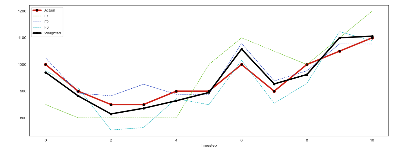
If our predictions are temporally ordered, i.e. forecasts or time series, then as time passes it is likely that we will see the relative performance of a model trend up or down. Several natural questions arise from this behavior.

1. How can we design an online algorithm to adjust relative weights of each model as their performance changes over time?
2. If we have multiple related time series, can we gain performance from combining each model uniquely for each forecast? Put another way, we might apply the technique to each time series individually, rather than the dataset as a whole. The example in this article will consider the case of forecasting visitors to many different restaurants. Other examples might be forecasting sales of many items across many stores or forecasting individual stocks in a mutual fund.

Thus this article will provide an exploration of several methods used to combine forecasts that will answer these questions. The majority of the focus will be on an approach based on AdaBoost and another using online projected gradient descent. We then apply each technique to forecasting restaurant visitors and assess the performance of each method. Finally, we give some extensions and commentary about these techniques.

Towards an Algorithm Inspired by AdaBoost

The goal of AdaBoost is to take weak hypotheses and combine them into a single, final hypothesis: \sum_{m=1}^{M}\alpha_{m}y_{m}(x), where m is the number of hypotheses, \alpha_{m} is the weight of the m^{th} hypothesis and y_{m}(x) is the prediction of the m^{th} hypothesis. Note that AdaBoost will find optimal \alpha_{m} and y_{m}(x) subject to the exponential error between y_{m}(x) and the true values Chapter 14.3 Pattern Recognition and Machine Learning - Bishop . However, the idea of weighting each final model is only half of the story of AdaBoost and actually is not what directly gives us our desired forecast weights. As a learning algorithm AdaBoost shines because each iteration it gives you a distribution of weights w_{n} for weighting the importance of each data instance. The way AdaBoost determines data instance weights is what will lead us to our algorithm for determining forecast ensemble weights.

Original AdaBoost Algorithm

Initialize weights, w_{n}^{(1)} = 1/N for n = 1,...,N, where N is the number of data instances

Create "weak" models, m=1,...,M:
   Fit model m, y_{m}(x) to minimize the error of weighted training data w_{n}^{(m)}
   Evaluate the model with the corresponding true values t_{n} to get error \epsilon_{m}
   Evaluate \alpha_{m} = log(\frac{1-\epsilon_{m}}{\epsilon_{m}})
   Update w_{n}^{(m+1)} = w_{n}^{(m)}exp(\alpha_{m}y_{m}(x))

Output \sum_{m=1}^{M}\alpha_{m}y_{m}(x)

With AdaBoost in mind, to get weights in a way that fits our problem there are some significant and non-obvious changes that have to be made. First, we need to see the difference in the problems we are trying to solve. AdaBoost at every iteration is creating a new model to add to the ensemble, based on the weights it assigns to each data instance. What we are interested in are just the weights w at every successive timestep. Since we will be breaking down our dataset into individual timesteps, we can focus on computing weights for one timestep at time for simplicity. This eliminates any loops for now. So our problem reduces to computing w_{n}^{(m+1)} given some initial weights and a new y_{m}(x) and t_{n} (for use in calculating the error). With this, we will follow the original algorithm where n will correspond to the number of our existing models (and thus the number of weights we will produce). The variable m will not come up, but it can be thought of as the amount of timesteps we will have to generate weights for.

Adaptive Weighting Algorithm

AdaWeight

Input: forecasts (f_{1},...,f_{n}), actual (float), learning\_rate (float), p (int), prior (p_{1},...,p_{n})

w_{n}^{(i)}= prior

\epsilon_{n} = |forecasts - actual|^{p} / Z, where Z is a normalization constant so \epsilon_{n} sums to 1.
\alpha_{n} = learning\_rate * log( \frac{1-\epsilon_{n}}{\epsilon_{n}})
w_{n}^{(i+1)} = w_{n}^{(i)} * exp(\alpha_{n}\epsilon_{n})/ Z, where Z is another normalization constant so w_{n}^{(i+1)} sums to 1.

return w_{n}^{(i+1)}

Here we have the pseudocode for AdaWeight. The algorithm starts by taking as input an array of forecast values each aimed at predicting actual. It takes in an array of prior weights which can be anything as long as they sum to 1. Prior can represent a previous output of AdaWeight (i.e. from the previous time step), it can represent an expectation of how each forecast will perform, or it could be a cold start where each weight is equal. Learning\_rate and p are hyperparameters that can be used to tune the resulting weights and some notes about their effects are described soon.

Initially, the algorithm sets the current weights w_{n} to the prior. It then calculates the absolute error \epsilon_{n} raised to the p power. The hyperparameter p can be thought of as a way to increase how much we amplify the best forecast, and deemphasize the weak. As p is increased, relatively good forecast's errors will stay relatively small, while bad forecast's errors will balloon higher much faster.

Once we have the error \epsilon_{n} AdaWeight finds \alpha_{n} as in the above pseudocode. Note that just like in the original AdaBoost, as \epsilon_{n} gets smaller, \alpha_{n} gets larger Yoav Freund and Robert E. Schapire. A short introduction to boosting. Journal of Japanese Society for Artificial Intelligence, 14(5):771--780, September, 1999. . The learning\_rate factor can either reduce this effect if it is < 1, or amplify the effect if> 1. The weights w_{n} are updated using the equation in the pseudocode. The effect of this is that if \alpha_{n} is relatively high, its resulting weight will also be higher. Thus we have achieved our goal of nudging up the weights of forecasts with relatively low errors and nudging down the weights of forecasts with relatively high errors. Finally, to achieve our original goal of adjusting weights at every timestep, we can iteratively call AdaWeight providing it the output of the previous call in the prior parameter.

Online Projected Gradient Descent

The Adaptive Weighting algorithm as presented in the previous section has a striking similarity to online gradient descent.

Online Gradient Descent

Initialize w_{n}^{(i)}

for i = 1,...,t-1:
 Get w_{n}^{(i)} and incur cost f^{(i)}(w_{n}^{(i)})
 w_{n}^{(i+1)} = w_{n}^{(i)} - \eta * \nabla f^{(i)}(w_{n}^{(i)})

return w_{n}^{(i+1)}

Breaking it down, we first notice how the loop here represents iterating over every timestep, so we can ignore it for now, since later we can just apply the algorithm iteratively to each new set of weights w.

Online Gradient Descent	AdaWeight
Get w_{n}^{(i)} Incur cost f^{(i)}(w_{n}^{(i)})	w_{n}^{(i)}= prior \epsilon_{n} = |forecasts - actual|^{p} / Z
nudge = \eta * \nabla f^{(i)}(w_{n}^{(i)}) w_{n}^{(i+1)} = w^{(i)} - nudge	\alpha_{n} = learning\_rate * log( \frac{1-\epsilon_{n}}{\epsilon_{n}}) w_{n}^{(i+1)} = w_{n}^{(i)} * exp(\alpha_{n}\epsilon_{n}) / Z

The first line is equivalent to having the prior (weights) available and then calculating the error \epsilon in AdaWeight. The second line is our “nudge” of the weights based on the gradient of the loss function. This is equivalent in AdaWeight to finding α and using it to nudge the weights using the exponential function. With this connection, all that remains to do is frame our problem as minimizing a convex function over a constraint set where the output vector's values need to be between 0 and 1 inclusive and sum to 1.

Similar to our power absolute error function in AdaWeight, we define our loss function for gradient descent as L_{x, a}(w) = |(xw-aw)^{p}| Proof that absolute value function raised to a power is convex. . . The subtle difference being that we calculate the error of each forecast x scaled by its weight w. This allows us to calculate the gradient with respect to the weights, with the weights being what we are trying to optimize. Framed in this way, our goal becomes to find a w that minimizes the absolute error of the weighted forecasts raised to some power (it will be 1 by default). The gradient with respect to w is \nabla L_{x, a}(w) = \frac{p(x-a)(xw-aw)^{2p-1}}{|(xw-aw)^{p}|}.

Now the question remains of how to project our weights after the nudge to ensure that we stay within our constraint set For more information on projected gradient descent see these notes from Hardt at Berkeley. . First we notice that our constraint set can be written as:

w^{T}\vec1 = 1 (weights sum to 1)
w \geq 0 (each weight is ≥ 0)

This is exactly the constraint set for a projection onto a probability simplex. Efficient algorithms exist to compute this projection, the algorithm Project comes from a short paper from UC MercedWang, Weiran, and Miguel Á. Carreira-Perpiñán. Projection onto the Probability Simplex: An Efficient Algorithm with a Simple Proof, and an Application. ArXiv:1309.1541 [Cs, Math, Stat], Sept. 2013. arXiv.org, http://arxiv.org/abs/1309.1541 .

Project

Input: \vec v\: \epsilon \; R^{D}

\vec u = sort \vec v descending
p = max{for j=1,...,D: u_{j} + \frac{1}{j}(1-\sum_{i=1}^{j}u_{i})}
\lambda = \frac{1}{p(1-\sum_{i=1}^{p}u_{i})}
\vec x = for i=1,...,D: x_{i} = max\{y_{i} + λ, 0\}

return \vec x

Using this projection function gives us the closest vector that is inside our constraint set in terms of the L2 norm. This is opposed to the naive approach of normalizing the data to sum to 1 and clipping negative values to 0, which would not give us such a statement of being optimal in terms of the L2 norm.

Putting the pieces together now gives us our final algorithm.

Online Projected Gradient Descent for Weighting

Input: x (x_{1},...,x_{n}), a (float), \eta (float), p (int), prior (p_{1},...,p_{n})

w_{n}^{(i)}= prior

w_{n}^{(i+1)} = w_{n}^{(i)} - \eta \nabla L_{x,a}(w_{n}^{(i)})
w_{n}^{(i+1)}= Project(w_{n}^{(i+1)})

return w_{n}^{(i+1)}

Testing on Synthetic Data

Here we will run AdaWeights and gradient descent on synthetic data to build intuition on how they work and as a sanity check to see if they behave as we expect.

Test 1

We generate forecasts from three different normal distributions. They will all be centered around the same true value, but with different standard deviations. This will represent one clear best forecast, SD10, one middle ground, SD25, and one clear worst, SD100. In this scenario we would expect to see the best forecast have a very high weight, the next best with a smaller weight, and the worst with a weight near zero, given enough iterations.

Figure 3: We see that both models do what we expect after running them for 1000 timesteps on the “forecasts” drawn from the normal distributions as described above. AdaWeights ends up setting the best forecast, SD10, to have a near 1 weight. Gradient descent interestingly converges to 0.7 for the best forecast and 0.3 for the second best.
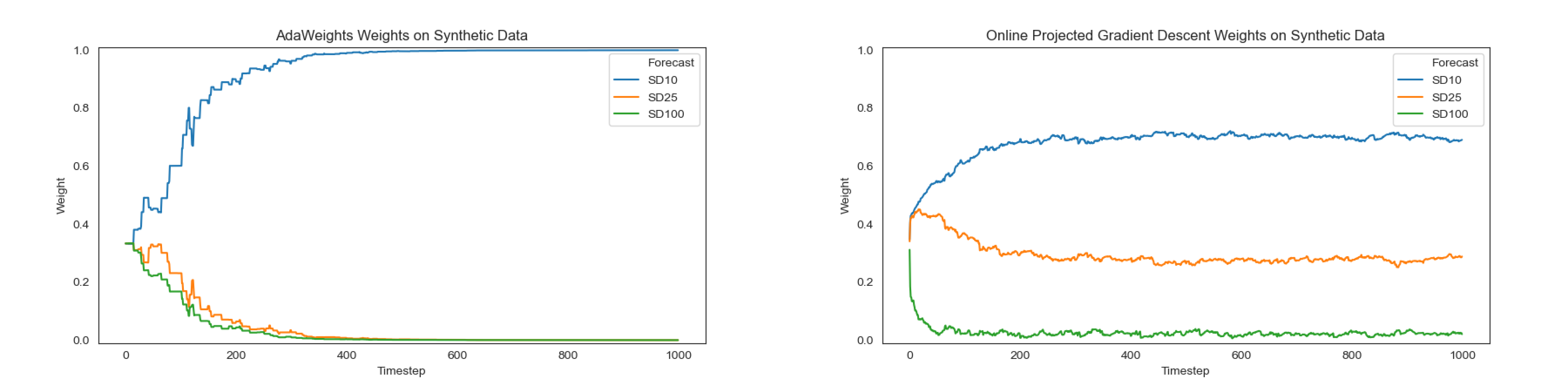
Note that both algorithms were run on the same synthetic data.

Test 2

Here we generate forecasts from three of the same normal distributions. Each is centered around 1000 with a standard deviation of 25. In this case we would likely want each forecast to be weighted similarly to maximize diversity in our ensemble.

We see that gradient descent performs in line with our expectations, with the weights of each forecast staying very close to each other. AdaWeights on the other hand does not have this behavior. It seems once one forecast has a good streak, it tends to keep that forecast’s higher and not converge back to even weighting until there is another very bad forecast by that model.
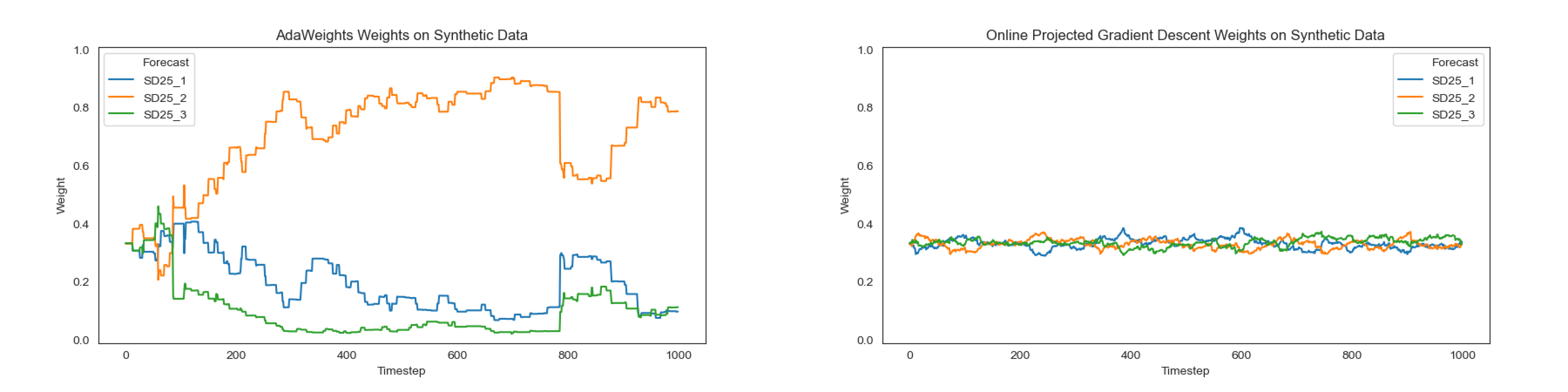
Note that both algorithms were run on the same synthetic data.

Stacking

Now that we have two optimization based algorithms, let's briefly look at a well-known method that leverages machine learning. Stacking, gaining fame from the top 2 Netflix prize solutions Netflix Prize Competition Sill, Joseph, et al. "Feature-Weighted Linear Stacking." ArXiv:0911.0460 [Cs], Nov. 2009. arXiv.org, http://arxiv.org/abs/0911.0460. , involves training a machine learning algorithm which uses the existing predictions as training data to generate a blended final target.

A basic procedure of how to use stacking.
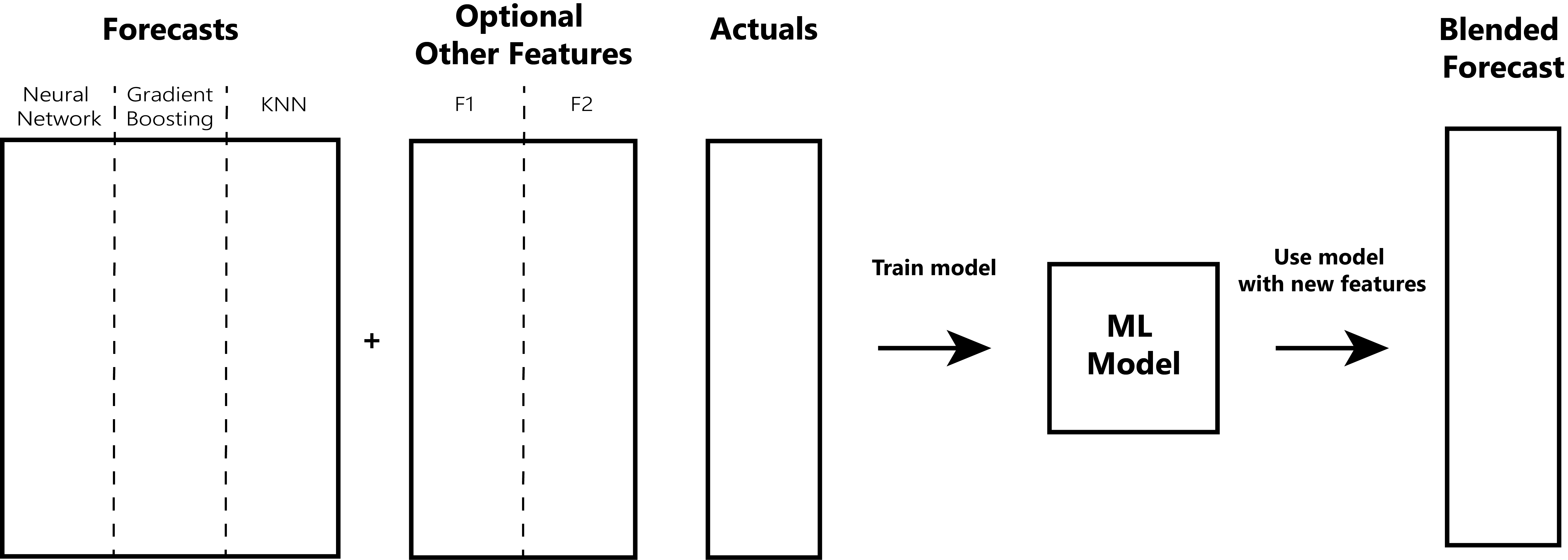
We have some set of forecasts we already generated and an optional dataset of associated features. These extra features can be anything that we think will help the blending model create a better prediction. These features combined with the target actuals are used to train a new model. We then use this trained model to generate a single, blended forecast (of course in practice we would provide it out of training sample data).

Practical Example

Now we turn to testing each algorithm on a real dataset, courtesy of an old Kaggle competition. The goal of the Recruit Restaurant Visitor Forecasting competition was to predict how many future visitors a restaurant/store will receive.

We took models from top performing kernels in order to get a variety of different forecasts to test our algorithms on. The first set of three models are based on the 8th place solution. They each use the features as described in that notebook (see Implementations and Code to Reproduce section for our code). All the models using these features are gradient boosting based. Two use Microsoft’s LightGBM and the other is XGBoost. For undetermined reasons, all three of these models underperformed overall, but we decided to keep them in as a good test of what happens if models start to perform poorly!

The second set of four models come from the notebook Exclude same wk res from Nitin's SurpriseMe2 w NN by Kaggle user Andy Harless. From this notebook we take 4 models that all use a different set of features compared to model set 1. The model families are GradientBoosting from Sklearn, KNN, XGBoost, and a feed forward neural network implemented using Tensorflow 2.

Instead of submitting our results to the competition to get the hidden scores, we opted to only use the provided data in order to be able to break down the problem into a more useful scenario. We generate forecasts using the models trained weekly rather than in one sequence of 39 days. For example, for the first period we stop training with data from before 2017-03-02. Then we generate predictions for the next seven days: 2017-03-04 to 2017-03-10. We repeat this process for the following 5 weeks of data, moving up the end of the training data each time. In this way, we prevent data leakage because a prediction for any day was made with data from at least two days before.

We apply each of the three previously discussed algorithms to the generated forecasts. Our baseline is to naively weight each model based on how they did overall on test data as it was described in the beginning of this article. For AdaWeight and gradient descent we create a matrix of weights that we use to apply to the set of forecasts two days into the future. So if AdaWeight’s last iteration was for 2017-04-02, then the weights it generated are applied to the forecasts for 2017-04-04. This can be thought of as lagging the generated weights by two days to ensure that we are not leaking data by using actuals to generate weights for that same day. In this way we ensure that we simulate a realistic environment since you would not have the actual value until at least the next day. The dataset consists of visitor counts to hundreds of stores. We treat each store as a separate time series, so the algorithm is applied from a "cold start" for each store in the dataset. We also note that we start off each algorithm with the prior set as the naive baseline weights.

For stacking we create a model trained on data from 2017-03-04 to 2017-03-27. The model we chose as the blender was LightGBM and used hyper parameters close to the defaults which are effective for many other problems. We also provide the model with two additional features, the store and the day.

Here is a comparison of how each individual model and each ensemble method performed tested on forecasts from 2017-03-29 to 2017-04-22. We use RMSLE as our metric as is done in the competition.

	RMSLE
GradientBoostingSklearn	0.54624
KNN	0.57193
LightGBM_1	0.60038
LightGBM_2	0.59961
Neural Network	0.49415
XGBoost_1	0.49881
XGBoost_2	0.58884
Naive Weighted	0.48753
AdaWeight	0.48801
Online Projected Gradient Descent	0.48826
Stacking w/LightGBM	0.54625

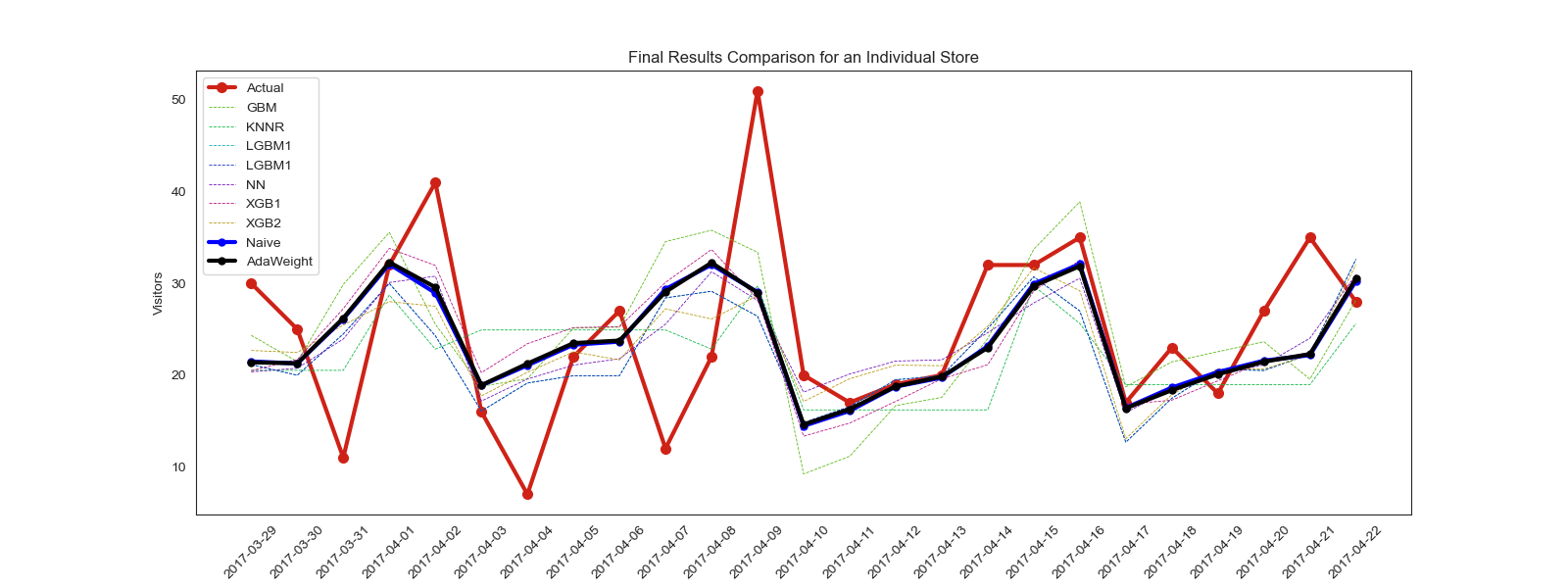
The tabular results show that AdaBoost and Gradient Descent are both essentially identical to the naively weighted solution and beat the best individual model by a fair margin. Stacking lags far behind doing about as well or worse than if each model was weighted evenly. In regards to the plot, it becomes more apparent that a good set of naive weights compared to the algorithm does not make a significant difference, positive or negative, in the overall results.

Extensions

The loss function chosen for the gradient descent algorithm is based on a combination of mean squared error and absolute error. There are likely other differentiable metrics that could be used for the minimization problem.
Similarly, in regards to AdaWeights, the error function could also be modified to have additional properties. One clever metric might be to take into consideration the pairwise bias of the forecasts. The intuition behind this is that just choosing the best single model is not optimal when you have one forecast above and another below the true value. In this scenario, you could find a weight that gives you exactly the point forecast. With this in mind, you might be more inclined to weight higher forecasts that are biased in opposite ways. In our current algorithm, two forecasts that are both biased in the same way (i.e. are nearly identical) are treated the same as two forecasts that are biased in opposite ways to each other. Perhaps put another way, it might be useful to find a metric that boosts diversity in your forecasts.

An intuitive optimization of both learning\_rate and p, outside of optimizing to cross-validation scores is to find values that limit the maximum weight change per iteration. A procedure might be to start with a low learning rate or low p value, and then increase it by a fixed step size until a weight changes by more than some amount, say 0.1. This gives a weak guarantee that your weights will not change too fast. The opposite optimization could be done starting from an initial learning rate where you see a change of more than some amount like 0.1. Then you lower the learning rate until you see no weight changes of more than 0.1 per iteration.

An interesting experiment would be to test prior weights and see how long takes for the prior to be irrelevant. Or in other words, how many iterations it takes until the weights starting with and without the prior are equal.

Conclusion

We presented two online algorithms for adjusting the relative weights of models as their performance changes over time. AdaWeights was inspired by the machine learning algorithm AdaBoost and utilized some of the mathematics behind it. The second was an application of online projected gradient descent, a method ubiquitous in continuous optimization. We also presented another common ensemble technique, stacking, to compare its results alongside. While AdaWeights and gradient descent did not have a large improvement over our naive baseline, they are still worthy considerations in problems where ensembling large amounts of models for many time series is required. We showed how each algorithm is able to automatically adjust weights of each forecast to keep up with its relative recent performance. Such a method could be invaluable in a scenario where it is infeasible for a human to monitor the performance of each model over every time series. These algorithms allow for a hands off approach to creating a blend of forecasts. Finally, we provide implementations and code to reproduce the experiments in the Github repository described below.

If you liked this article, consider reading my first article on a method for correcting forecast errors based on it’s previous errors. If you want to be informed of other data science and machine learning news head over to mlfeed.tech or follow MLTwitterFeed on Twitter.

Implementations and Code to Reproduce

Code implementing AdaWeights and gradient descent and code to reproduce the various experiments and models can be found on Github. It was written and tested using Python 3.7.4 64-bit on Windows and a list of package requirements is provided in requirements.txt.

• Algorithm implementations are in optimization.py.
• Using these algorithms and how to recreate the experimental results using them is in the jupyter notebook AdaWeighting.ipynb.
• Code to create the feature engineered datasets and models used to generate the predictions used can be found in mk_datasets.py.
• Code to generate the predictions can be found in mk_predictions.py.
• Code for creating the various figures used in this article is located in Figures.ipynb.