Introduction
Standard machine learning models: gradient boosting, multilayer perceptron, random forecast, etc have no implicit notion of time. The order of the training data is irrelevant and they treat each sample as independently and identically distributed (i.i.d.). Of course, temporal features can be added such as hour, weekday, month, and so on depending on the specific problem. However, it still is likely that the model will exhibit temporal bias. Intuitively, temporal bias is when a short series of consecutive predictions consistently under or over forecast the true value, while the model as a whole may exhibit no such bias. The latter is especially the case with high capacity models like gradient boosting or multilayer perceptron. This article describes a method called Moving Average Correction (MAC) which aims to correct for short-term temporal biases.
Problem Formulation
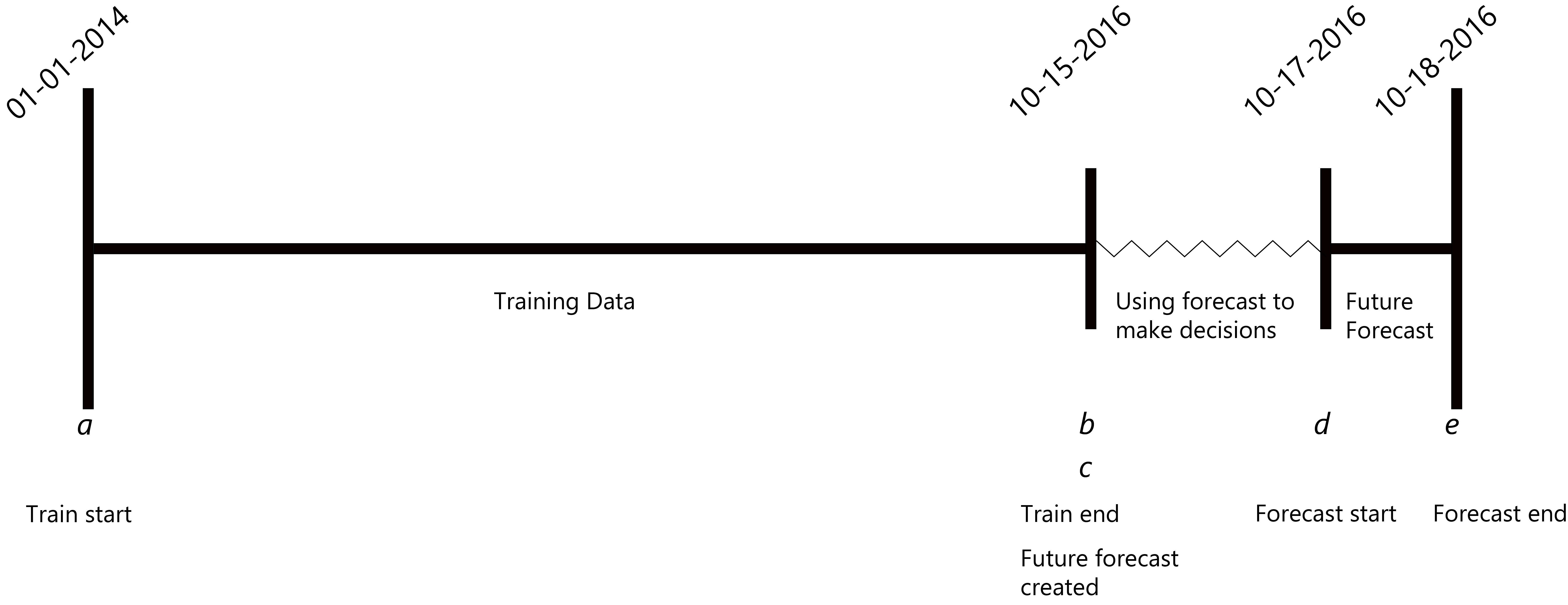
Using machine learning for forecasting, especially multivariate, is extremely common. Many of these problems can be more formally defined as using some amount of historical data from time a to time b to train a model. At time c we use the model to generate predictions using data available at time c to generate a forecast for time d to time e. Note that the times must be ordered a ≤ b ≤ c ≤ d ≤ e. See Figure 1 illustrating this for a toy example.
General Examples
- Server load
- When more servers might need to be provisioned or determining good times to perform operations that might reduce overall server capacity
- Estimating the amount of motor vehicle collisions
- Help determine how much trauma and EMS support will be needed.
See NYC Open Data
NYC Open Data: Motor Vehicle Collisions - Crashes for an interesting dataset that can be used to do this - Future product demand
- Determining how much of a product will be needed. Can be on either end, either for selling to some consumer, or how much is expected to be needed for manufacturing
- Energy demand forecasting
- How much electricity people are going to use
Toy Example
The running toy example in this article will be predicting future hourly traffic for a particular roadway in New
York City.
The dataset can be found from NYC Open Data
MAC Algorithm
At its core, MAC is calculating the average error over some historical period, then adding the inverse of those average errors to the future period.
We first need to have some notion of periods. For example, if we are predicting a value for every hour and we do this for the entire next day, this would constitute one period: 24 values corresponding to each hour. Input to the algorithm is a forecast for one period in the future. The output will correspond to the MAC future forecast. The algorithm also needs as input a historical forecast alongside its corresponding true values. This should be one or more consecutive historical periods. Note that it generally will make most sense to pick the x periods closest to the future period. The algorithm will calculate an error corresponding to each instance in a period and then add the inverse of those errors to the future period.
Algorithm in Psuedocode
Input: HF: consecutive historical forecast broken up into periods
Input: AF: a matching, consecutive actual forecast broken up into periods
Input: FF: one future forecast period
errors = list of size period of errors
Iterating over every period in HF and AF in parallel*:
Find the average error at the current index i,
errors[i] = avg(HF[i] - AF[i]) (where HF[i] and AF[i] are column vectors)
Apply errors to FF,
FF = FF - errors
return FF
*HF and AF are now matrices where each column is a slice in time (e.g. an hour) and each row is a different period.
MAC Visualized in Three Cases
Case 1
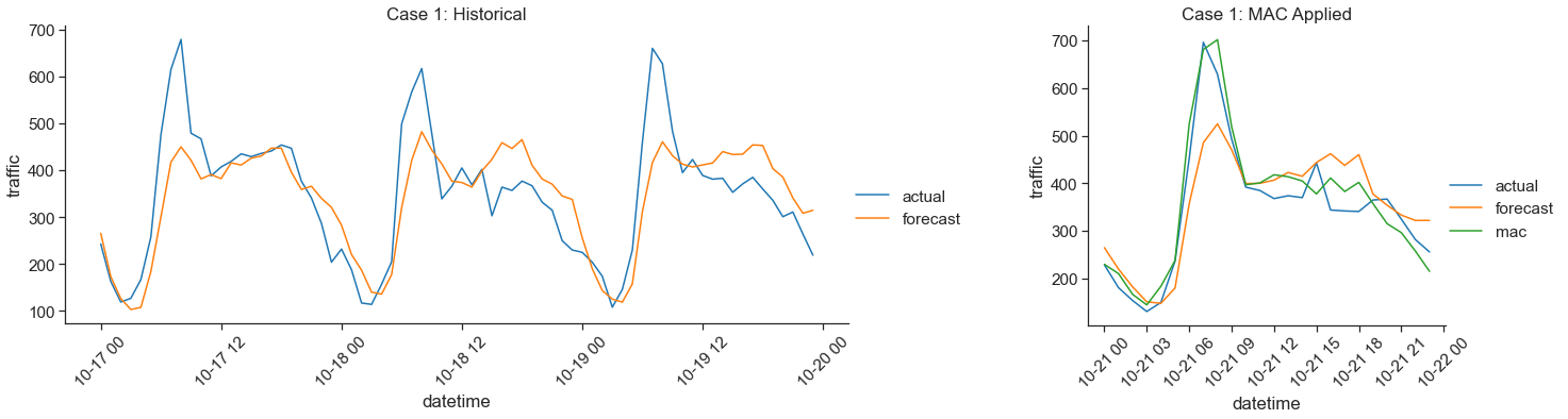
When observing the output of a forecast over a few consecutive periods it is common to see that the forecast is consistently over or under the true value. In this case, the respective over or under forecasting continues into the future. This is the best case scenario for MAC as it will always get you closer to the true value.
Here we predict traffic on Broadway, southbound from West 174th Street to West 175th Street. In the morning hours the LightGBM forecast was significantly off each day by similar amounts. This trend continued to the forecast for 10-21 and led to a significant improvement in forecast errors. The mean absolute error of the historical forecast was 61.8, the future forecast (without MAC) was 51.8 and the MAC future forecast was 33.8.
Case 2
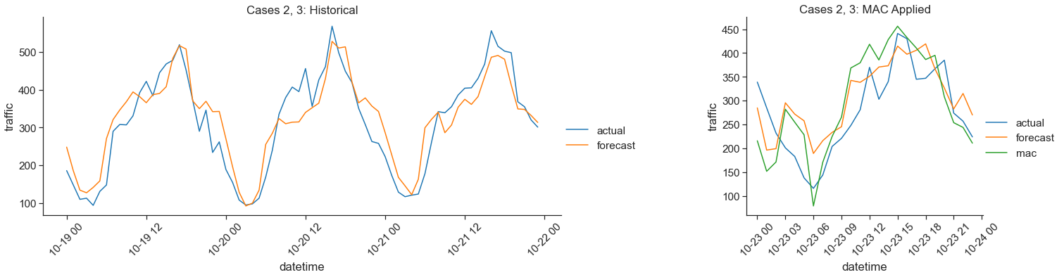
The worst case scenario for MAC is the direct opposite of case 1. The historical forecast is showing consistent over or under forecasting, but then it changes to the other for the future day. Ex. The historical periods were consistently under, but then the future period is over. This means that the MAC forecast will be even more wrong.
Case 3
The final case is a neutral case for MAC where it does not change much the output of the future forecast. The historical forecast is either consistently accurate or sometimes over and sometimes under. In this case, the average errors will either be close to zero or cancel out so the future forecast is not affected much.
Here we predict traffic on Broadway, northbound from West 174th Street to West 175th Street. The application to Case 2 here is that at around hour 12 we see a slight trend of under forecasting, but then on the future day the forecast was very close to the true value at that time, so the MAC future forecast was worse. The application to Case 3 is that generally across the historical hours, there is not a consistent bias that the historical forecast exhibits, so therefore the MAC future forecast is close to the future forecast itself.
The mean absolute error of the historical forecast was 43.7, the future forecast (without MAC) was 54.7 and the MAC future forecast was 58.4.
Intuition Summarized
The assumption that enables MAC to do well is that the bias in the forecast is going to continue into the future. In general, this may be a good assumption to make. Often it is difficult for a machine learning model trained on tens of thousands of samples to pick up on a change that is just becoming present in a small amount of the most recent data. Effectively, MAC bridges the gap between wanting to use as much data as possible, while also being robust to sudden changes in the new data distribution.
Extensions
In conclusion, we showed how to formulate a problem in a way that is reasonable to apply MAC. We then gave a description of the method and how it can perform when various cases happen in the forecast. MAC still has plenty of potential to be extended and tuned to the specific problem at hand.
Exponential Moving Average: In vanilla MAC we use a standard moving average, treating each historical period as
contributing equal amounts to the error score and we only consider a fixed set of periods in the past. The amount
of
past periods is a tunable parameter. A straightforward adaptation would be to use an exponential moving average
Instead of using the exact average error, a “MAC smoothing factor” factor could be applied. This would simply take the errors found by MAC and scale them up or down by a constant factor. For example, if the error for a particular instance in a period was 100 and the MAC smoothing factor was 0.5, then the error applied to the future forecast would be 50.
Example Code in a Jupyter Notebook
Code implementing MAC for the toy example can be found on
Github in
MAC_NYC.ipynb. It includes the data sets, formatting the data,
the baseline lightgbm model used, and the code for the plots. The notebook can be directly viewed at the link or
the repository can be cloned. A list of package requirements is provided in requirements.txt and has
been tested using Python 3.7.4 64-bit on Windows.